Simple Finance Prediction using Deep Learning

Currently, a significant amount of financial negotiations are already made by computers, which take into account several factors (news, market turmoil, past quotations) and try to predict future movements of the assets. These algorithms add liquidity money to the market.

This project is a just simple prediction using Deep Learning. The data used for training and network accuracy testing are historical data that it was got from Yahoo finance. The libraries used in this project were Pandas, Tensorflow, numpy and others.

The neural network was designed to predict the quotation of the day using the past 30 adj. close (the features). However, it does not make much sense to judge the network based only on the adj. close price, because many factors can influence the closing value. This neural network has two internal layers, the first with 10 and the second with five neurons, the learning rate of 0.001, with cost function Mean Squared Error, iterating 7000 times. The modification of the biases’ layers are constant and the weight uses the normal distribution with 0 mean and 0.1 of standard deviation.

Feedfoward Neural Network CODE

The feedforward neural network was the first and simplest type of artificial neural network devised. In this network, the information moves in only one direction, forward, from the input nodes, through the hidden nodes (if any) and to the output nodes. There are no cycles or loops in the network.

# FEEDFORWARD NEURAL NETWORK
n_nodes_hl1 = 10
n_nodes_hl2 = 5

n_classes = 1

batch_size = x_train.shape[0]
hm_epochs = 7000

x = tf.placeholder('float')
y = tf.placeholder('float')

def neural_network_model(data):
    hidden_1_layer = {'f_fum': n_nodes_hl1,
                      'weight': tf.Variable(tf.truncated_normal([len(x_train[0]), n_nodes_hl1], mean=0.0, stddev=0.1)),
                      'bias': tf.Variable(tf.constant(0.1, shape=[n_nodes_hl1]))}

    hidden_2_layer = {'f_fum': n_nodes_hl2,
                      'weight': tf.Variable(tf.truncated_normal([n_nodes_hl1, n_nodes_hl2], mean=0.0, stddev=0.1)),
                      'bias': tf.Variable(tf.constant(0.1, shape=[n_nodes_hl2]))}

    output_layer = {'f_fum': None,
                    'weight': tf.Variable(tf.truncated_normal([n_nodes_hl2, n_classes], mean=0.0, stddev=0.1)),
                    'bias': tf.Variable(tf.constant(0.1, shape=[n_classes])), }

    l1 = tf.add(tf.matmul(data, hidden_1_layer['weight']), hidden_1_layer['bias'])
    l1 = tf.nn.relu(l1)

    l2 = tf.add(tf.matmul(l1, hidden_2_layer['weight']), hidden_2_layer['bias'])
    l2 = tf.nn.relu(l2)

    output = tf.add(tf.matmul(l2, output_layer['weight']), output_layer['bias'])

    return output

# TRAIN NEURAL NETWORK

def train_neural_network(x):
    prediction = neural_network_model(x)

    cost = tf.reduce_mean(tf.squared_difference(prediction, y))
    optimizer = tf.train.AdamOptimizer(learning_rate=0.001).minimize(cost)

    with tf.Session() as sess:
        sess.run(tf.global_variables_initializer())


        for epoch in range(hm_epochs):
            epoch_loss = 0
            i = 0
            while i + batch_size <= len(x_train):
                start = i
                end = i + batch_size
                batch_x = np.array(x_train[start:end])
                batch_y = np.array(y_train[start:end])
               

                _, c = sess.run([optimizer, cost], feed_dict={x: batch_x,
                                                              y: batch_y})
                epoch_loss += c
                i += batch_size

            print('Iteração %4d' % (epoch + 1), 'de', hm_epochs, 'Erro:', epoch_loss)
            epoch += 1

        out = sess.run([prediction], feed_dict={x: x_test})

Results

#=> prints MSE:  [16.22116169] and Accuracy:  68.98550724637681 %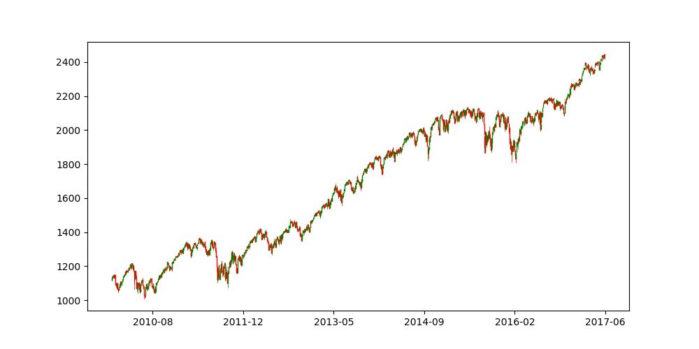

This plot is a candle stick plot of the data

This plot is a style of financial chart used to describe price movements of a security, derivative, or currency.

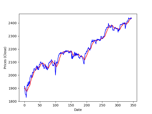
It is the prediction plot. the blue line is the adj. close of the data and the red line is the prediction of the adj. close

Conclusion

Obviously, there is still a lot of work to be done. There are several other trial options. We can also goal the trend of the market which in this case is the best option, or use indicators such as moving average and use other features, or even create networks that analyze news and identify whether the market is optimistic or pessimistic. This is just a simple project that uses Tensorflow on Financial Market, but in my opinion, all the possibilities to use Deep Learning on the financial market are fascinating.

“Just as electricity transformed almost everything 100 years ago, today I actually have a hard time thinking of an industry that I don’t think Artificial Intelligence will transform in the next several years.” - Andrew NG